UnPivot or Reverse Pivot Data

I just found out that PivotTable and PivotChart Wizard can be used to ‘Unpivot’ or ‘Reverse Pivot’ in Excel.

I will explain the procedure by UnPivotting the table shown below.

PivotTable and PivotChart Wizard won’t be available in the Excel Ribbon or Quick Access Toolbar by default. You need to manually add this feature to the QAT to access it. For that Right-click on the Quick Access Toolbar and select Customize Quick Access Toolbar. In the Excel Options Dialog, Select All Commands from the drop-down menu under the label choose commands from:

Select PivotTable and PivotChart Wizard from the available options and add it to Quick Access Toolbar

Now we have the button for PivotTable and PivotChart Wizard in QAT.

Click on PivotTable and PivotChart Wizard

Select the option called Multiple Consolidation range from the Dialog and Click on Next

Select the option I will create the Page Fields and Click on Next

Specify the address of the data range containing data in the new dialog, Click on Add and then Next

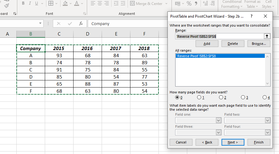
Specify the location where you want to place the Pivot Table Report and Click on Finish. Here I will be placing the Pivot Table Report in the cell B10 of the Existing worksheet.

Now we have a Pivot Table Report at the cell B10

Remove the fields for Row form the Rows and Column from Columns and that will give us a single cell containing the Grand Total of values.

Double-click (Drill-Down) on the cell to see the entire records which constitute to this value. Following is the Unpivotted form of the table which we started with.